Spatial autocorrelation

ㅤSpatial autocorrelation refers to a clustering pattern in the spatial distribution of a variable, indicating the extent to which a variable is spatially correlated with itself. Positive autocorrelation (or clustering) occurs when neighboring observations are more similar to each other, while negative autocorrelation (or dispersion) occurs when neighboring observations tend to differ. This technique can be divided into two main methods:

• Global Spatial Autocorrelation
• Local Spatial Autocorrelation

Spatial weight

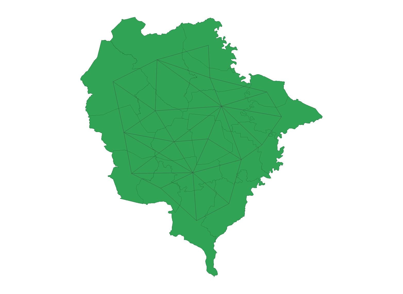
ㅤIn the first step, we identify the spatial weight matrix $(W)$ as a square binary matrix based on queen contiguity. The concept of queen contiguity considers adjacent neighbors that mutually share borders and edges. In this square binary matrix, if units i and j share a border, the matrix weight $(w_{ij})$ is set to 1; if they do not share a border,$(w_{ij})$ is set to 0. The diagonal elements of the weight matrix $(w_{ii})$ are also set to 0. In this study, Spatial weight of 18 locations(sub-district) was evaluated and calculated queen contiguity by using GeoDa (version 1.22) as presented in the figure below.

Global Spatial Autocorrelation

ㅤA global detection technique was used to assess spatial autocorrelation across the entire study area, providing a single summary measure that describes the overall degree of spatial association in the dataset. The Global Moran’s I statistic (Moran, 1950) was used to calculate the global autocorrelation coefficient. It yields a score ranging between -1 and 1: a positive score indicates clustering of similar values, a negative score indicates dispersion of similar values, and a score close to zero suggests a random spatial distribution.

Global Moran’s I statistic equation is ¹:

$$I = \frac{n}{S_0} \cdot \frac{\sum_{i=1}^{n} \sum_{j=1}^{n} w_{ij} (x_i - \bar{x})(x_j - \bar{x})}{\sum_{i=1}^{n} (x_i - \bar{x})^2}$$
Where:

• \(I\) is the Global Moran’s I for observation \(i\).
• \(n\) is the total number of observations.
• \(x_i\) and \(x_j\) are the values of the variable of interest at locations \(i\) and \(j\).
• \(\bar{x}\) is the mean of the variable of interest.
• \(w_{ij}\) is the spatial weight between locations \(i\) and \(j\).
• \(S_0 = \sum_{i=1}^{n} \sum_{j=1}^{n} w_{ij}\)

ㅤInference for Global Moran’s I was based on the null hypothesis of spatial randomness. The significance of the Global Moran’s I statistic was evaluated using a permutation test distribution, with 99,999 random permutations computed using GeoDa (version 1.22).

Local Spatial Autocorrelation

ㅤLocal detection focuses on spatial autocorrelation at specific locations within the study area. The Local Moran’s I statistic was used to calculate local autocorrelation. A positive Local Moran’s I indicates a cluster of similar values, while a negative Local Moran’s I indicates clustering of dissimilar values. If the Local Moran’s I is close to zero, it suggests that there is no significant spatial clustering at that location.

Local Moran’s I statistic equation is ²:

$$I_i = \frac{\sum_{j=1}^{n} w_{ij} (x_i - \bar{x})(x_j - \bar{x})}{\sum_{i=1}^{n} (x_i - \bar{x})^2}$$
Where:

• \(I_i\) is the Local Moran’s I for observation \(i\).
• \(x_i\) is the value of the variable of interest at location \(i\).
• \(x_j\) is the value of the variable at location \(j\).
• \(\bar{x}\) is the mean of the variable of interest.
• \(w_{ij}\) is the spatial weight between location \(i\) and location \(j\).
• \(\sum_{i=1}^{n} (x_i - \bar{x})^2\) is the total sum of squared deviations from the mean.

ㅤThe significance of the Local Moran’s I statistic for each spatial unit was evaluated using a permutation test distribution, with 99,999 random permutations computed using GeoDa (version 1.22). This high number of permutations increases the precision of the significance tests, ensuring more reliable identification of significant spatial clusters. Results are considered significant when the p-value is less than 0.05.

Local Indicators of Spatial Association (LISA)

ㅤLocal Indicators of Spatial Association (LISA), as described by Anselin (1995), are used to identify the magnitude of spatial clustering around specific geographical points or areal units. Each observation reveals the extent of significant spatial clustering of similar values in the vicinity of that location. In this study, LISA was utilized to analyze local spatial autocorrelation, which resulted in four distinct categories²:

• High-High Clusters: Areas where high values cluster with other high values.
• Low-Low Clusters: Areas where low values cluster with other low values.
• High-Low Outliers: Areas with high values surrounded by low values.
• Low-High Outliers: Areas with low values surrounded by high values.

ㅤThis classification helps to understand the spatial distribution of the variable of interest and identify patterns of spatial dependence within the study area.

Moran scatter plot

ㅤThe Moran scatter plot, introduced by Anselin (1996), plots the spatially lagged variable on the y-axis and the original variable on the x-axis. The slope of the linear fit represents Moran’s I. For a variable $Z$ in deviations from the mean and row-standardized weights where $S_0$ equals the number of observations $N$, Moran’s I simplifies to³:

$$I = \frac{\sum_i \sum_j w_{ij} z_i z_j}{\sum_i z_i^2} = \frac{\sum_i (z_i \times \sum_j w_{ij} z_j)}{\sum_i z_i^2}$$

In this context, the slope of the regression of $\sum_j w_{ij} z_j$ on $z_i$ represents Moran’s I.

Inference

Null hypothesis

ㅤPermutation inference for Moran’s I relies on a null hypothesis of spatial randomness, with the statistic’s distribution derived either under the assumption of normality (independent normal random variates) or randomization (where each value is equally likely at any location)³.

Pseudo p-value

ㅤThe reference distribution is used to calculate a pseudo p-value as³:

$$p = \frac{R + 1}{M + 1}$$ Where:

• \(p\) is the pseudo p-value.
• \(R\) is the number of times the computed Moran's I from permuted data is equal to or more extreme than the observed statistic.
• \(M\) is the number of permutations.

Reference

(1) Bivand RS, Wong DW. Comparing implementations of global and local indicators of spatial association. Test. 2018;27(3):716-48.

(2) Anselin L. Local indicators of spatial association—LISA. Geogr Anal. 1995;27(2):93-115

(3) GeoDa Center for Geospatial Analysis and Computation. Global Spatial Autocorrelation (Lab 5A). Available at: https://geodacenter.github.io/workbook/5a_global_auto/lab5a.html. [Accessed 8 September 2024.]